Computing gradients in parallel with Amazon Braket
Published: December 8, 2020. Last updated: November 6, 2024.
Note
Go to the end to download the full example code.
PennyLane integrates with Amazon Braket to enable quantum machine learning and optimization on high-performance simulators and quantum processing units (QPUs) through a range of providers.
In PennyLane, Amazon Braket is accessed through the PennyLane-Braket plugin. The plugin can be installed using
pip install amazon-braket-pennylane-plugin
A central feature of Amazon Braket is that its remote simulator can execute multiple circuits in parallel. This capability can be harnessed in PennyLane during circuit training, which requires lots of variations of a circuit to be executed. Hence, the PennyLane-Braket plugin provides a method for scalable optimization of large circuits with many parameters. This tutorial will explain the importance of this feature, allow you to benchmark it yourself, and explore its use for solving a scaled-up graph problem with QAOA.

Why is training circuits so expensive?
Quantum-classical hybrid optimization of quantum circuits is the workhorse algorithm of near-term quantum computing. It is not only fundamental for training variational quantum circuits, but also more broadly for applications like quantum chemistry and quantum machine learning. Today’s most powerful optimization algorithms rely on the efficient computation of gradients—which tell us how to adapt parameters a little bit at a time to improve the algorithm.
Calculating the gradient involves multiple device executions: for each trainable parameter we must execute our circuit on the device typically more than once. Reasonable applications involve many trainable parameters (just think of a classical neural net with millions of tunable weights). The result is a huge number of device executions for each optimization step.

In the standard default.qubit device, gradients are calculated in PennyLane through
sequential device executions—in other words, all these circuits have to wait in the same queue
until they can be evaluated. This approach is simpler, but quickly becomes slow as we scale the
number of parameters. Moreover, as the number of qubits, or “width”, of the circuit is scaled,
each device execution will slow down and eventually become a noticeable bottleneck. In
short—the future of training quantum circuits relies on high-performance remote simulators and
hardware devices that are highly parallelized.
Fortunately, the PennyLane-Braket plugin provides a solution for scalable quantum circuit training by giving access to the Amazon Braket simulator known as SV1. SV1 is a high-performance state vector simulator that is designed with parallel execution in mind. Together with PennyLane, we can use SV1 to run in parallel all the circuits needed to compute a gradient!
Accessing devices on Amazon Braket
The remote simulator and quantum hardware devices available on Amazon Braket can be found
here. Each
device has a unique identifier known as an
ARN. In PennyLane,
all remote Braket devices are accessed through a single PennyLane device named braket.aws.qubit,
along with specification of the corresponding ARN.
Note
To access remote services on Amazon Braket, you must first create an account on AWS and also follow the setup instructions for accessing Braket from Python.
Let’s load the SV1 simulator in PennyLane with 25 qubits by specifying the device ARN.
device_arn = "arn:aws:braket:::device/quantum-simulator/amazon/sv1"
SV1 can now be loaded with the standard PennyLane device():
import pennylane as qml
from pennylane import numpy as np

n_wires = 25

dev_remote = qml.device(
    "braket.aws.qubit",
    device_arn=device_arn,
    wires=n_wires,
    parallel=True,
)
Note the parallel=True argument. This setting allows us to unlock the power of parallel
execution on SV1 for gradient calculations. We’ll also load default.qubit for comparison.
dev_local = qml.device("default.qubit", wires=n_wires)
Note that a local Braket device braket.local.qubit is also available. See the
documentation for more details.
Benchmarking circuit evaluation
We will now compare the execution time for the remote Braket SV1 device and default.qubit. Our
first step is to create a simple circuit:
def circuit(params):
    for i in range(n_wires):
        qml.RX(params[i], wires=i)
    for i in range(n_wires):
        qml.CNOT(wires=[i, (i + 1) % n_wires])

    # Measure all qubits to make sure all's good with Braket
    observables = [qml.PauliZ(n_wires - 1)] + [qml.Identity(i) for i in range(n_wires - 1)]
    return qml.expval(qml.prod(*observables))

In this circuit, each of the 25 qubits has a controllable rotation. A final block of two-qubit CNOT gates is added to entangle the qubits. Overall, this circuit has 25 trainable parameters. Although not particularly relevant for practical problems, we can use this circuit as a testbed for our comparison.
The next step is to convert the above circuit into a PennyLane QNode().
qnode_remote = qml.QNode(circuit, dev_remote)
qnode_local = qml.QNode(circuit, dev_local)
Note
The above uses QNode() to convert the circuit. In other tutorials,
you may have seen the qnode() decorator being used. These approaches are
interchangeable, but we use QNode() here because it allows us to pair the
same circuit to different devices.
Warning
Running the contents of this tutorial will result in simulation fees charged to your AWS account. We recommend monitoring your usage on the AWS dashboard.
Let’s now compare the execution time between the two devices:
import time

params = np.random.random(n_wires)

t_0_remote = time.time()
qnode_remote(params)
t_1_remote = time.time()

t_0_local = time.time()
qnode_local(params)
t_1_local = time.time()

print("Execution time on remote device (seconds):", t_1_remote - t_0_remote)
print("Execution time on local device (seconds):", t_1_local - t_0_local)
Execution time on remote device (seconds): 7.571744918823242
Execution time on local device (seconds): 27.32159185409546
Nice! These timings highlight the advantage of using the Amazon Braket SV1 device for simulations
with large qubit numbers. In general, simulation times scale exponentially with the number of
qubits, but SV1 is highly optimized and running on AWS remote servers. This allows SV1 to
outperform default.qubit in this 25-qubit example. The time you see in practice for the
remote device will also depend on factors such as your distance to AWS servers.
Note
Given these timings, why would anyone want to use default.qubit? You should consider
using local devices when your circuit has few qubits. In this regime, the latency
times of communicating the circuit to a remote server dominate over simulation times,
allowing local simulators to be faster.
Benchmarking gradient calculations
Now let us compare the gradient-calculation times between the two devices. Remember that when
loading the remote device, we set parallel=True. This allows the multiple device executions
required during gradient calculations to be performed in parallel, so we expect the
remote device to be much faster.
First, consider the remote device:
d_qnode_remote = qml.grad(qnode_remote)

t_0_remote_grad = time.time()
d_qnode_remote(params)
t_1_remote_grad = time.time()

print(
    "Gradient calculation time on remote device (seconds):",
    t_1_remote_grad - t_0_remote_grad,
)
Gradient calculation time on remote device (seconds): 6.4775872230529785
Now, the local device:
Warning
Evaluating the gradient with default.qubit will take a long time, consider
commenting-out the following lines unless you are happy to wait.
d_qnode_local = qml.grad(qnode_local)

t_0_local_grad = time.time()
d_qnode_local(params)
t_1_local_grad = time.time()

print(
    "Gradient calculation time on local device (seconds):",
    t_1_local_grad - t_0_local_grad,
)
Gradient calculation time on local device (seconds): 181.5902488231659
Wow, the local device needs around 3 minutes! Compare this to less around 6 seconds spent calculating the gradient on SV1. This provides a powerful lesson in parallelization.
What if we had run on SV1 with parallel=False? It would have taken around 3 minutes—still
faster than a local device, but much slower than running SV1 in parallel.
Scaling up QAOA for larger graphs
The quantum approximate optimization algorithm (QAOA) is a candidate algorithm for near-term quantum hardware that can find approximate solutions to combinatorial optimization problems such as graph-based problems. We have seen in the main QAOA tutorial how QAOA successfully solves the minimum vertex cover problem on a four-node graph.
Here, let’s be ambitious and try to solve the maximum cut problem on a twenty-node graph! In maximum cut, the objective is to partition the graph’s nodes into two groups so that the number of edges crossed or ‘cut’ by the partition is maximized (see the diagram below). This problem is NP-hard, so we expect it to be tough as we increase the number of graph nodes.

Let’s first set the graph:
import networkx as nx

nodes = n_wires = 20
edges = 60
seed = 1967

g = nx.gnm_random_graph(nodes, edges, seed=seed)
positions = nx.spring_layout(g, seed=seed)

nx.draw(g, with_labels=True, pos=positions)

We will use the remote SV1 device to help us optimize our QAOA circuit as quickly as possible. First, the device is loaded again for 20 qubits
dev = qml.device(
    "braket.aws.qubit",
    device_arn=device_arn,
    wires=n_wires,
    parallel=True,
    max_parallel=20,
    poll_timeout_seconds=30,
)
Note the specification of max_parallel=20. This means that up to 20 circuits will be
executed in parallel on SV1 (the default value is 10).
Warning
Increasing the maximum number of parallel executions can result in a greater rate of spending on simulation fees on Amazon Braket. The value must also be set bearing in mind your service quota.
The QAOA problem can then be set up following the standard pattern, as discussed in detail in the QAOA tutorial.
cost_h, mixer_h = qml.qaoa.maxcut(g)
n_layers = 2
def qaoa_layer(gamma, alpha):
qml.qaoa.cost_layer(gamma, cost_h)
qml.qaoa.mixer_layer(alpha, mixer_h)
def circuit(params, **kwargs):
for i in range(n_wires): # Prepare an equal superposition over all qubits
qml.Hadamard(wires=i)
qml.layer(qaoa_layer, n_layers, params[0], params[1])
return qml.expval(cost_h)
cost_function = qml.QNode(circuit, dev)
optimizer = qml.AdagradOptimizer(stepsize=0.01)
We’re now set up to train the circuit! Note, if you are training this circuit yourself, you may want to increase the number of iterations in the optimization loop and also investigate changing the number of QAOA layers.
Warning
The following lines are computationally intensive. Remember that running it will result in simulation fees charged to your AWS account. We recommend monitoring your usage on the AWS dashboard.
import time

np.random.seed(1967)
params = 0.01 * np.random.uniform(size=[2, n_layers], requires_grad=True)
iterations = 10

for i in range(iterations):
    t0 = time.time()

    params, cost_before = optimizer.step_and_cost(cost_function, params)

    t1 = time.time()

    if i == 0:
        print("Initial cost:", cost_before)
    else:
        print(f"Cost at step {i}:", cost_before)

    print(f"Completed iteration {i + 1}")
    print(f"Time to complete iteration: {t1 - t0} seconds")

print(f"Cost at step {iterations}:", cost_function(params))

np.save("params.npy", params)
print("Parameters saved to params.npy")
Initial cost: -29.98570234095953
Completed iteration 1
Time to complete iteration: 11.028863906860352 seconds
Cost at step 1: -29.995107300982195
Completed iteration 2
Time to complete iteration: 10.132628917694092 seconds
Cost at step 2: -29.99981056829394
Completed iteration 3
Time to complete iteration: 9.985284090042114 seconds
Cost at step 3: -30.00233965117029
Completed iteration 4
Time to complete iteration: 10.059210062026978 seconds
Cost at step 4: -30.01206799710033
Completed iteration 5
Time to complete iteration: 9.966963052749634 seconds
Cost at step 5: -30.048670540725286
Completed iteration 6
Time to complete iteration: 11.216133832931519 seconds
Cost at step 6: -30.13240170461342
Completed iteration 7
Time to complete iteration: 10.09446096420288 seconds
Cost at step 7: -30.25935979157505
Completed iteration 8
Time to complete iteration: 10.020287990570068 seconds
Cost at step 8: -30.41499293575487
Completed iteration 9
Time to complete iteration: 10.345153093338013 seconds
Cost at step 9: -30.587353834845057
Completed iteration 10
Time to complete iteration: 10.07306981086731 seconds
Cost at step 10: -30.76855713404487
Parameters saved to params.npy
This example shows us that a 20-qubit QAOA problem can be trained within around 1-2 minutes per
iteration by using parallel executions on the Amazon Braket SV1 device to speed up gradient
calculations. If this problem were run on default.qubit without parallelization, we would
expect for training to take much longer.
The results of this optimization can be investigated by saving the parameters
here to your working directory. See if you can
analyze the performance of this optimized circuit following a similar strategy to the
QAOA tutorial. Did we find a large graph cut?
Large-scale experiments with Hybrid Jobs
We have seen how we can use PennyLane on Braket to solve graph optimization problems with QAOA. However, we have only used Amazon Braket for the quantum simulations, leaving the classical Python code to run on our laptop. This is great for getting started with small experiments, but for large-scale algorithms running them on a laptop is impractical due to potential crashes, restarts or even hardware limitations such as limited memory. With Amazon Braket Hybrid Jobs, you can send your entire algorithm, both classical and quantum parts, to run on AWS while you get a coffee!
With a single line of code, we’ll see how to scale from PennyLane simulators on your laptop to run full-scale experiments on AWS that leverage both powerful classical compute and quantum devices. For more details on hybrid jobs see getting started with hybrid jobs.
Warning
The following demo is only compatible with Python version 3.10.
In the following code, we run the same QAOA optimization as before, but this time on an Amazon EC2 ml.c5.xlarge instance instead of our laptop. We specify this with the instance_config for our hybrid job. A complete set of options is available in the Braket documentation.
from braket.jobs import InstanceConfig, hybrid_job
from braket.jobs.metrics import log_metric
from braket.tracking import Tracker

# choose a large instance type for our experiment
large_instance = InstanceConfig(instanceType="ml.c5.xlarge")


@hybrid_job(device="local:pennylane/lightning.qubit", instance_config=large_instance)
def qaoa_training(n_iterations, n_layers=2):
    braket_tasks_cost = Tracker().start()  # track Braket quantum tasks costs

    # declare PennyLane device
    dev = qml.device("lightning.qubit", wires=n_wires)

    @qml.qnode(dev)
    def cost_function(params, **kwargs):
        for i in range(n_wires):  # Prepare an equal superposition over all qubits
            qml.Hadamard(wires=i)
        qml.layer(qaoa_layer, n_layers, params[0], params[1])
        return qml.expval(cost_h)

    params = 0.01 * np.random.uniform(size=[2, n_layers])
    optimizer = qml.AdagradOptimizer(stepsize=0.01)

    # run the classical-quantum iterations
    for i in range(n_iterations):
        params, cost_before = optimizer.step_and_cost(cost_function, params)

        log_metric(metric_name="cost", value=cost_before, iteration_number=i)

    return {
        "parameters": params,
        "final_cost": cost_function(params),
        "braket_tasks_cost": braket_tasks_cost.qpu_tasks_cost()
        + braket_tasks_cost.simulator_tasks_cost(),
    }
Now we create a hybrid job by calling the function as usual. This returns an AwsQuantumJob
object that contains the device ARN, region, and job name. The hybrid job will start running
immediately since we are not using a QPU in this example.
Warning
Running the the following cell will result charges to your AWS account based on Amazon EC2 pricing.
job = qaoa_training(n_iterations=20, n_layers=2)
print(job)
AwsQuantumJob('arn':'arn:aws:braket:<aws-region>:<account_id>:job/qaoa-training-1695044583')
The hybrid job automatically captures the function arguments as hyperparameters.
In this case, we set n_iterations = 20 and n_layers = 2 as the hyperparameters.
We can check the status with:
job.state()
'QUEUED'
The hybrid job will be scheduled to run and will appear in the “QUEUED” state. If the target is a QPU, the job will be queued with other jobs. If the target device is not a QPU, the hybrid job should start immediately. Note that since the algorithm code is run in a containerized environment, it takes approximately 1 minute to start running your algorithm.
After the hybrid job is completed, we can get the results with job.result(). For this example,
it should take approximately 6 minutes.
job.result()
{'parameters': [[-0.2615367426048209, -0.46218141633156967],
                [0.3853200394389563, 0.2402391372931216]],
 'final_cost': -37.76176577995996,
 'braket_tasks_cost': 0}
The results included the three values from the return statement of our function. Additionally, we can retrieve the metrics recorded during the training with:
metrics = job.metrics()
Now that we have the metrics, we can plot the convergence of the loss function. We use the pandas library to load the metrics into a DataFrame, and plot the loss as a function of iteration number.
import pandas as pd
import matplotlib.pyplot as plt

plt.style.use("pennylane.drawer.plot")

df = pd.DataFrame(metrics)

df.sort_values(by=["iteration_number"]).plot(x="iteration_number", y="cost")

Great! The loss function gets lower with each iteration, reaching a value of approximately -37.8.
Conclusion
In this tutorial, we found the solution to a MaxCut problem using QAOA. We used Amazon Braket on-demand simulators to efficiently parallelize the parameter-shift rule for gradients. We also demonstrated how to scale-up experiments with your own simulator, such as PennyLane Lightning, by running on Amazon Braket Hybrid Jobs. In both approaches, we perform the intensive calculations on the cloud instead of our laptop.
For more examples of how to use hybrid jobs, see the Amazon Braket examples GitHub.
Maria Schuld
Dedicated to making quantum machine learning a reality one day.
Matthew Beach
Matthew Beach is an Applied Scientist at Amazon Braket. His research focuses on the intersection of machine learning and quantum physics with an emphasis on using computational methods to study many-body systems.
Share demo